Lately you can’t shut me up about hybrid search. The core problem retrieval engines have in hybrid search boils down to getting a healthy set of candidates that represent the best vector candidates that also match lexically
Essentially hybrid search can become a big chicken + egg problem. I’ve talked about solving this with filters, but in reality we can’t do this forever. Filtered vector search is slow (or not available!). The complexity explodes to the cartesian product of every lexical attribute.
Let’s look for a better way before our chickens come home to roost.

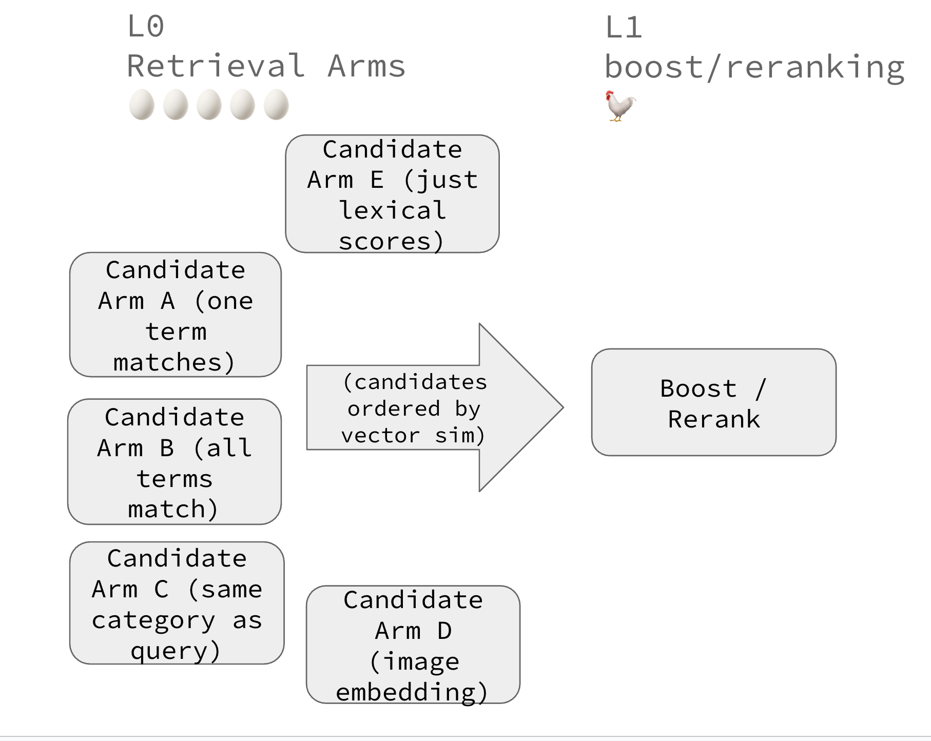
In most search engines, the 🥚 left hand (egg) part looks something like this psuedo-SQL below. Some selection of lexical candidates (here by ‘garden trowel’ matching some text), then ordered by vector similarity from a vector index, giving us a first pass rough ranking.
SELECT * FROM <search>

-- FILTER to these lexical candidates before similarity search
WHERE  (garden in product_name OR garden in product_description OR
        trowel in product_name OR trowel in product_description)

-- SORT by embedding similarity
ORDER BY vector_similarity(query_embedding, title_embedding)

-- TOP N CANDIDATES within this set
LIMIT 100
Now in the 🐓 RHS (chicken) part, we can manipulate the best lexical AND vector candidates in some reranker or boosts.
Of course, we probably want many types of candidates, that match different lexical criteria. So our chickens eventually lay waaay to many eggs to be manageable:
SELECT * FROM <search>

-- FILTER to these lexical candidates before similarity search
WHERE  (garden in product_name OR garden in product_description OR
        trowel in product_name OR trowel in product_description)

-- SORT by embedding similarity
ORDER BY vector_similarity(query_embedding, title_embedding)

-- TOP N CANDIDATES within this set
LIMIT 100

UNION ALL

SELECT * FROM <search>

-- FILTER to these lexical candidates before similarity search
WHERE  ("lawn and garden" in department)

-- SORT by embedding similarity
ORDER BY vector_similarity(query_embedding, title_embedding)

-- TOP N CANDIDATES within this set
LIMIT 100

UNION ALL

...
You can see how this gets unmanagable…
(I showed some examples in Elasticsearch with the WANDS dataset in my previous blog post)
More arms, more problems
Many of us start with a simple pretrained embedding model for the first pass vector retrieval. We often don’t revisit this… until its too late.
As we select more types of candidates, the more crowded the L0 (🥚) becomes. Performance and complexity suffers.
Perhaps we should collapse more query/doc attributes into our embedding itself? Then our early ranking need not select for so many types of lexical candidates?
One way to do this is with a two-tower model. It learns an embedding from our ground truth (ie a judgment list) with the document/query attributes as inputs.
IE something like this:
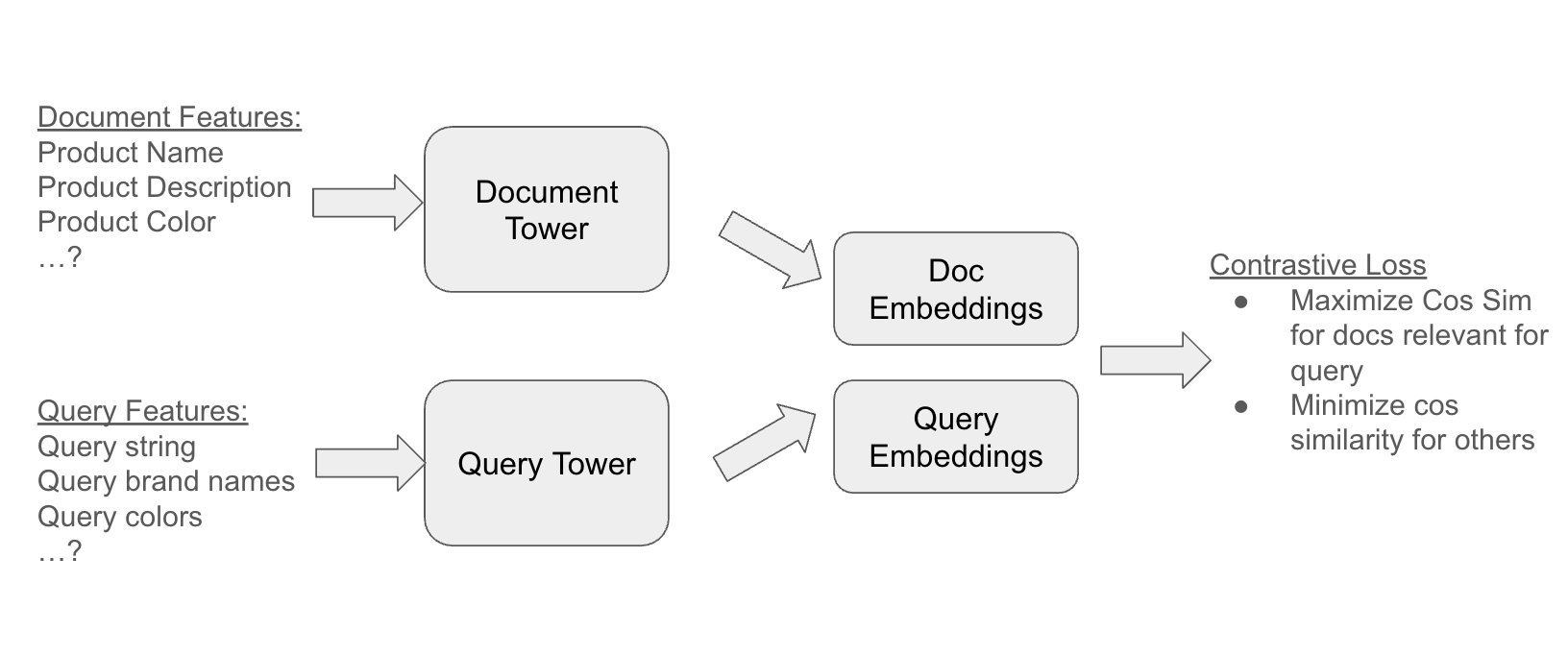
We identify product and query features (here just strings). They’re then fed through essentially two parallel models - or towers. The document tower learning an embedding of the document, query tower the query embedding.
But the real power is the final step - the contrastive loss - specific to our training data. We move closer embeddings from each tower that are positive examples. We move apart all other examples.
| Query | Document | Relevant? | Contrastive Loss: |
|---|---|---|---|
| red shoe | 👠 | 1 | Move query/doc embeddings CLOSER |
| red shoe | 🩰 | 1 | Move query/doc embeddings CLOSER |
| red shoe | 👖 | 0 | Move query/doc embeddings FARTHER |
Now we should see query embeddings grow more similar to their relevant document counterparts, and vice-versa.
Break down some code to me like I’m 5
Well you’re in luck, because I act like I’m 6, so I can probably explain to a 5 year old.
Here’s some actual code to follow along.
First, we need to take strings → tokenized representation. This representation is actually for transformer oriented use cases, we get the tokenizer from the transformers library:
tokenizer = AutoTokenizer.from_pretrained("distilbert-base-uncased")
We run with batches, getting 16 or so instances of queries, names, product descriptions:
queries = list(batch[0])
product_names = list(batch[1])
product_descriptions = list(batch[2])
Which we also tokenize in batches:
query_tokens = tokenizer(queries, padding=True, truncation=True, return_tensors="pt").to(device)
product_name_tokens = tokenizer(product_names, padding=True, truncation=True, return_tensors="pt").to(device)
product_description_tokens = tokenizer(product_descriptions, padding=True, truncation=True, return_tensors="pt").to(device)
Each of these is a python dictionary. Having key input_ids - the numerical id of a token, ie maybe the is token 1234 or something in the transformer’s vocabulary. And attention_mask - basically a 1 to indicate to the model a token is here, otherwise padded to 0.
The model itself
The model itself, crucially has inside of it a text_encoder - the pretrained transformer model from transformers library.
self.text_encoder = AutoModel.from_pretrained(model_name) # model name distilibert
This is just a pretrained transformer layer…
When we run the forward pass (ie we’re not training yet, just pushing inputs through), we pass the earlier tokenized text (remember input_ids/attention_mask), in. This generates a BERT embedding:
def encode_text(self, encoded):
    output = self.text_encoder(encoded['input_ids'], attention_mask=encoded['attention_mask'])
    # Use CLS token representation
    return output.last_hidden_state[:, 0, :]
Then in our model’s train method, we do this to both the document’s name and product. We tack on a fully-connected layer with weights for each embedding dimension against itself. IE a weight for how dimension 123 should apply to 567, etc. These weights become the main thing being learned.
doc_features = []
name_embedding = self.encode_text(product_token_features['product_name'])
name_embedding = self.product_name_proj(name_embedding)
doc_features.append(name_embedding)

description_embedding = self.encode_text(product_token_features['product_description'])
description_embedding = self.product_description_proj(description_embedding)
doc_features.append(description_embedding)

...
# Stack / take mean product name and description embeddings
doc_emb = torch.stack(doc_features, dim=0).mean(dim=0)
doc_emb = self.doc_proj(doc_emb)
Here product_name_proj is just a 768 x 768 matrix, a fully connected layer to learn to weigh the transformers output.
Combining the towers
The full graph looks something like this:
[Product Description Text]
↓
[Tokenizer]
↓
[Transformer]  -- (frozen or lightly fine-tuned) -->  768-dim CLS vector
↓
[Projection Layer (Linear)] -- (trainable from scratch) -->  new 768-dim vector
↓
But in reality we have one of these also for the product name, and the next step is
↓
[Stack with other features]
[Combine (take mean?)]
I won’t repeat this whole thing for the query, but it follows the same path. In the end, the forward pass returns:
return query_emb, doc_emb
Finally contrastive loss, the diagonals are the examples of relevant results.
def contrastive_loss(query_emb, doc_emb, temperature=0.05):
    scores = torch.matmul(query_emb, doc_emb.t()) / temperature
    labels = torch.arange(scores.size(0)).to(scores.device)
    return nn.CrossEntropyLoss()(scores, labels)
Simply put
- matmul is the cosine similarity, over query and doc embeddings (transposed)
- labels here are all just “1” as we are showing only relevant examples
- Contrastive loss computes a loss where the direct examples should move closer in similarities, the other combinations like query_emb[0] with doc_emb[1] would move farther apart.
But nothing has actually been “updated” yet. All this is just a big computational graph, with weights at each stage that need to be learned.
Then through the magic of pytorch tensors, we backprop to learn those weights
query_emb, doc_emb = model(query_tokens, product_text_tokens)
loss = contrastive_loss(query_emb, doc_emb)
loss.backward()
optimizer.step()
The code runs this on the full WANDS (Wayfair e-commerce) dataset. I’ll leave it to you to run and play with.
Collapse the arms
Now with an embedding model, our eggs can turn into better chickens! OK strained metaphor. But we can:
- Even if we keep many of our mandatory filters, we will filter out much less, leading to faster vector search
- We’ll select better candidates at each arm for later usage by subsequent boosts / rerankers
- We’ll train our retrieval on our own training data, tailoring an embedding to our most important use-cases
Let me know your thoughts! Get in touch if I can help your team with a hybrid search project.
Enjoy softwaredoug in training course form!
Starting May 18!
Signup here - http://maven.com/softwaredoug/cheat-at-search I hope you join me at Cheat at Search with Agents to learn use agents in search. build better RAG and use LLMs in query understanding.

Doug Turnbull
More from DougTwitter | LinkedIn | Newsletter | Bsky