In the previous post, I demonstrated a pure Python algorithm for random-projections based locality-sensitive hashing (LSH) (code here). It’s a pretty simple way to try to compress floating point vectors into a bitmask to recover cosine similarity.
We saw… pretty terrible results. Middling recall. And single digit / low double digit QPS. Pretty bad.
Now, the algorithm itself has problems:
- It requires a linear scan of an array to get the most similar hashes to the query hash
- It recovers a similarity which is a different task than recovering nearest neighbors
This last point is a subtle but important one about vector search: Some neighbors may be very close, and tiny screwups in similarities can transport us to another neighborhood in a big city by just jumping a few blocks. But we don’t have this problem in a rural area, where people spread out, and similarity estimation is fine enough.
That crap implementation, tho…
But, perhaps more fundamentally, we had a dumb, pure Python implementation. So in this article, I want to create a Numpy-based C solution for processing our arrays of hashes.
I’m going to dive right in, I suggest you read the previous article for context. But the TL; DR, we’re working with hashes of vectors. You can read the last article to learn how we get these hashes. But know that hashes, to us, means bit array. They correspond to the vectors we’ve indexed. Our query, of course, corresponds to the hash of the query vector:
hash1: 0100
hash2: 1011
...
hashN: 0011
query: 1011
The hash that shares the most bits with the query corresponds to that with the highest cosine similarity. Finding that nearest hash - FAST - is our mission, and yes, we choose to accept it 🕵️♀️.
To find that hash, last time, we learned this one weird bit-twiddling trick. We can recover the number of unshared bits by doing this:
num_bits_set_to_1(hash XOR query) # fewer 1 bits (more 0 bits) on exclusive-or means closer similarity
Or, by example, XOR’ing (operator ^ in C and Python) the above hashes with query:
               XOR    UNSHARED: num_bits_set_to_1(XOR)
hash1 ^ query: 1111   4       # LEAST similar
hash2 ^ query: 0000   0       # MOST similar
hashN ^ query: 1100   2       # 2nd most
We say that hash2 is most similar to query. XOR’d together, they have the fewest 1s. Fewest unshared bits; most shared. And if you look at them, indeed they are exactly the same.
I’m going implement the entire algorithm in C. Essentially:
for each hash
    sim = num_bits_set_to_1( hash ^ query )      # you saw this before
    if sim < worst_sim_in_queue:                 # Save if more similar than what we've seen already
        insert sim into queue
This function gets some top N most similar (lowest is most similar) and maintains a queue, only inserting if the sim we compute is better than the worst thing in our top N.
Importantly, we will use the CPU popcount instruction to count bits instead of our earlier bit-twiddling method. Something exposed through compiler intrinsics in clang and GCC.
Setting up the C Numpy function
(I’m skipping the numpy tutorial on writing ufuncs. “Universal Functions” (ufuncs) are just custom C Numpy code for processing arrays. But highly suggested)
The Numpy UFunc itself looks like this. We’ll just look at it this one time, because it really just converts array arguments from numpy/python to the C variables I need:
static void hamming_top_n(char **args, const npy_intp *dimensions,
                          const npy_intp *steps, void *data)
{
    npy_intp num_hashes = dimensions[1];  /* appears to be size of first dimension */
    npy_intp query_len = dimensions[2];  /* appears to be size of second dimension */
    uint64_t *hashes = __builtin_assume_aligned((uint64_t*)args[0], 16);
    uint64_t *query =  __builtin_assume_aligned((uint64_t*)args[1], 16);
    uint64_t *query_start = __builtin_assume_aligned((uint64_t*)args[1], 16);
    uint64_t *best_rows = __builtin_assume_aligned((uint64_t*)args[2], 16);

    # discussed below
    hamming_top_n_default(hashes, query, query_start, num_hashes, query_len, best_rows);
The important thing to note in our python / numpy associated plumbing:
- Numpy preallocates arrays of input and output. We just populate the output (here
best_rows) - We get the
dimensionsof each item in an array, so we can use it safely - We get the Python args in
args. Herehashesandqueryare our array arguments from Python. IE you would call this function from Pythonhamming_top_n(hashes, query) - Later on when initializing this Ufunc we tell numpy the dimensions of valid input through the signature. We tell numpy our function has a sigature of
(m,n),(n) -> (10). Hashes would be (m,n), Query is an array of n, and we return 10. You can see where we do that here. - We also tell numpy that the input / output will be
uint64arrays, we do that on this line.
So in short, numpy knows exactly how to allocate and manage the arrays we get as input/output. We just need to transform input to output!
The algorithm in C – first pass
The first C implementation just calls: hamming_top_n_default:
void hamming_top_n_default(uint64_t* hashes, uint64_t* query, uint64_t* query_start,
                           uint64_t num_hashes, uint64_t query_len, uint64_t* best_rows) {
    struct TopNQueue queue = create_queue(best_rows);
    uint64_t sum = 0;
    for (uint64_t i = 0; i < num_hashes; i++) {
        sum = 0;
        query = query_start;
        for (uint64_t j = 0; j < query_len; j++) {
            sum += popcount((*hashes++) ^ (*query++));
        }
        /* Only add to output if its better than worst thing in our top 10*/
        maybe_insert_into_queue(&queue, sum, i);
    }
}
I’ll omit the maybe_insert_into_queue as it does not dominate performance. It just keeps our queue up to date if and only if sum (which is our similarity) is less than the current least-similar in the queue. You can check it out here
The code that dominates performance is this inner hot loop:
        for (uint64_t j = 0; j < query_len; j++) {
            sum += popcount((*hashes++) ^ (*query++));
        }
As our hashes can be > 64 bits, we sum the similarities of all of our hashes with the corresponding place in the hash.
If we build and run a benchmark of Glove 300 dimension vectors from the repo:
make test
python benchmark/glove.py pure_c 64 128 256 512 640 1280 2560
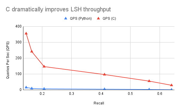
We get a pretty huge improvement from the pure Python implementation:
64 projections -- QPS 355.0464873171851 -- Recall 0.136499999999998
128 projections -- QPS 241.46964706002143 -- Recall 0.19549999999999798
256 projections -- QPS 146.8177150077879 -- Recall 0.283999999999999
512 projections -- QPS 130.2396482333485 -- Recall 0.38470000000000054
640 projections -- QPS 96.629607995171 -- Recall 0.4202000000000004
1280 projections -- QPS 55.37952621776572 -- Recall 0.5329
2560 projections -- QPS 29.13870808612148 -- Recall 0.6328999999999989
Graphed against the Python version, we get a pretty insane speedup. Still not anything competitive, but it shows just how crazy it costs to have the Numpy roundtrips between C and Python:
Unrolling some loops
The next thing I tried that worked was unrolling some of the loops. The cost of the loop counter, etc, was a large percentage of the instructions being executed for the smaller sized hashes (ie 64 or 128 bits / two uint64_ts).
So for the lower hash sizes, I created an alternate implemtation, based on this C macro:
#define HAMMING_TOP_N_HASH(N, BODY) \
void hamming_top_n_hash_##N(uint64_t* hashes, uint64_t* query, \
                          uint64_t num_hashes, uint64_t* best_rows) { \
    struct TopNQueue queue = create_queue(best_rows); \
    uint64_t sum = 0; \
    NPY_BEGIN_ALLOW_THREADS \
    for (uint64_t i = 0; i < num_hashes; i++) { \
      BODY; \
      maybe_insert_into_queue(&queue, sum, i); \
    } \
    NPY_END_ALLOW_THREADS \
}
This creates functions like hamming_top_n_hash_1, etc where BODY is the unrolled contents of the query to hash computation. Instead of a loop, its just the one line copy-pasted:
/* 64 bits */
HAMMING_TOP_N_HASH(1,
    sum = popcount((*hashes++) ^ (*query));
)

/* 128 bits */
HAMMING_TOP_N_HASH(2,
    sum = popcount((*hashes++) ^ (*query));
    sum += popcount((*hashes++) ^ query[1]);
)

/* 192 bits */
HAMMING_TOP_N_HASH(3,
    sum = popcount((*hashes++) ^ (*query));
    sum += popcount((*hashes++) ^ query[1]);
    sum += popcount((*hashes++) ^ query[2]);
)

...
(C Programmers please get in touch if there’s a smarter way to unroll than copy pasting these lines ;) ).
Then in the body of the top-level numpy function, we just choose which implementation to use after getting the args, defaulting to our earlier implementation if we don’t have an unrolled version for query_len.
    switch (query_len) {
        case 1:
            hamming_top_n_hash_1(hashes, query, num_hashes, best_rows);
            return;
        case 2:
            hamming_top_n_hash_2(hashes, query, num_hashes, best_rows);
            return;
        ...
        default:
            hamming_top_n_default(hashes, query, query_start, num_hashes, query_len, best_rows);
            return;
With these dumb performance hacks, does QPS improve? Yeah boi! This provided a significant performance speedup, especially for the lower sized hashes!
64 projections -- QPS 840.2823049187605 -- Recall 0.1289999999999998
128 projections -- QPS 594.8292691966128 -- Recall 0.193
256 projections -- QPS 365.12440313724113 -- Recall 0.25200000000000006
512 projections -- QPS 194.034303547326 -- Recall 0.40800000000000003
640 projections -- QPS 146.14705980853586 -- Recall 0.41000000000000014
1280 projections -- QPS 57.83595190887417 -- Recall 0.5739999999999997
2560 projections -- QPS 38.97597500828167 -- Recall 0.6549999999999996
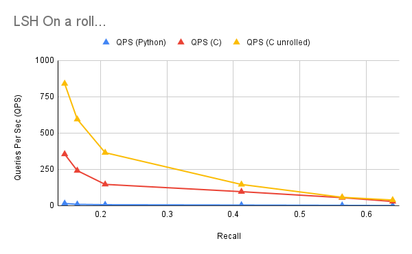
You’ll note the higher number of hashes, unrolling barely helps. As the cost of executing the loop counter / checking is small relative to the summing. So it becomes closer to the regular performance. As such, we don’t unroll much past 10 (640 projections).
But wait there’s cores more!
One thing we haven’t done is see if we can speed this up through just using all the cores on our CPU. Right now the above stats are a single core solution. Unfortunately, if we just throw this code behind the Python threading and issue multiple queries at once, things actually get slower?
Why is that? Well if you know Python, you know about the dreaded GIL. Since every search is behind a single Python call, it locks out concurrent calls from occuring.
Luckily I’m usually trustworthy when it comes to threading, and I feel this function is probably threadsafe. So we’ll use this little incantation that Numpy / CPython to tell it to disable the GIL. This lets usn search the hashes concurrently from multiple threads. CPython gives us a little macro.
All we need to do is wrap the outer loop accordingly:
void hamming_top_n_default(uint64_t* hashes, uint64_t* query, uint64_t* query_start,
                           uint64_t num_hashes, uint64_t query_len, uint64_t* best_rows) {
    struct TopNQueue queue = create_queue(best_rows);
    uint64_t sum = 0;
    NPY_BEGIN_ALLOW_THREADS
    for (uint64_t i = 0; i < num_hashes; i++) {
        sum = 0;
        query = query_start;
        for (uint64_t j = 0; j < query_len; j++) {
            sum += popcount((*hashes++) ^ (*query++));
        }
        /* Only add ot output if its better than nth_so_far. We don't care about sorting*/
        maybe_insert_into_queue(&queue, sum, i);
    }
    NPY_END_ALLOW_THREADS
}
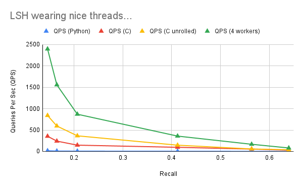
Running this under 4 worker threads gives us another significant performance improvement:
64 projections -- QPS 2395.0580356424443 -- Recall 0.12969999999999815
128 projections -- QPS 1556.6209180039205 -- Recall 0.19139999999999796
256 projections -- QPS 870.3183265554875 -- Recall 0.2803999999999986
512 projections -- QPS 499.93975726613667 -- Recall 0.3816000000000004
640 projections -- QPS 358.7610832214154 -- Recall 0.41790000000000066
1280 projections -- QPS 167.48470966960681 -- Recall 0.5302000000000001
2560 projections -- QPS 81.02739932963804 -- Recall 0.6396999999999985
Hitting limits of LSH
We can maybe make this a touch faster(?). But we are hitting limits of what’s possible with this algorithm. After all recall is not going up! And our best solution still is only 81 QPS.
What might be a next step?
As we said at the beginning - this algorithm attempts to recover the cosine similarity. It does not attempt to find the nearest neighbors. To actually recover nearest neighbors we have to begin to be parametric. In other words, we need to be sensitive to the structure of the data.
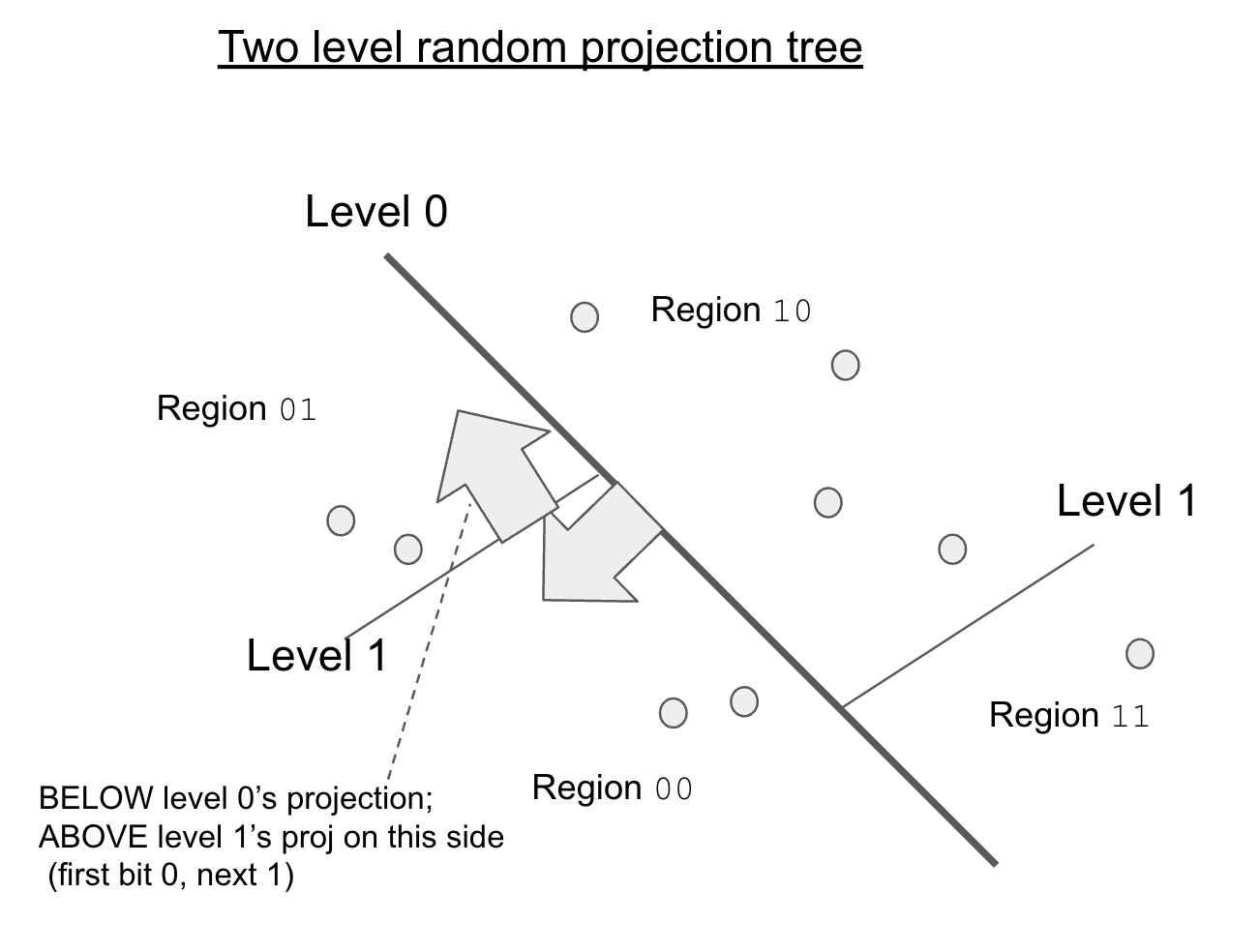
One possible next step would be a system like Annoy, which uses random projection trees.
What does it do differently?
First it chooses splits between two known data points. A subtle, but important point, as it allows the projections to essentially become biased. Instead of a random set of projections, our projections become warped to the data. Creator of Annoy - Erik Bernhardsen - has a nice presentation on random projections. But this also means the projections no longer help recover cosine similarity. That’s OK, if we just care about nearest neighbors: a block in New York is like 10 KM in rural Kansas.
Second it partitions the space up using a tree. So that we’re not breaking up the entire vector space each step. This is essentially what a KD-Tree does, except we’re using random projections into the data, rather some value on than the axes themselves.
Here’s a diagram showing the projections, notice the splits depend on the level.
Another possible step might be to use a different LSH technique like spectral hashing. Spectral hashing uses the principal components of the vector space to arrive at a better hash function. Another way of saying this: we notice on our earth that variation in latitude/longitude is more important than altitude in determining a neighbor. This is handy as instead of focusing on random projections: we use the dimensions we know are most important.
The hard thing about nearest-neighbors search…
All of these approaches share a big downside: we will need to periodically retrain and restructure our data globally sense to continue accurately recovering nearest neighbors. If, say, a global pandemic happens, and everyone moves out of a big city – the fundamental structure of the distribution of people changes. The postal service might update / create new zip codes. New area codes might need to be invented.
That’s the big tradeoff of vector search. If you want accurate nearest neighbors, your ability to accurately update an index becomes harder over time. You get drift. Eentually you will need to relearn the newest global state. Unlike indexing text, nearest neighbor search, fundamentally, requires us to evolve with the overall distribution of vectors themselves.
So again, it seems sometimes advantageous to have less recall, but simpler operational costs. Perhaps a dumb hashing function would be good enough on the right datasets? We wouldn’t have to retrain and can incrementally update without the headaches of periodic retraining / reconciling the global view of the vector space.
What do you think? Please hit me up with feedback!
Upcoming course: Build your own vector database

Want to understand what makes embedding retrieval fast, relevant, and useful in real AI systems? Join Build your own vector database and build the core pieces yourself, from embeddings and indexing to search and retrieval.

Doug Turnbull
More from DougTwitter | LinkedIn | Newsletter | Bsky