A pure python LSH nearest neighbors implementation

Like many search developers, my hobby is nearest-neighbors search. Ann-benchmarks has the latest-and-greatest vector databases vying for supremacy.

But… SCIENCE🔬!

I like to learn about the classic, boring old algorithms. Those missing from the leaderboard. The stuff nobody uses anymore but we could still learn from. Not because they’re “good” – though maybe they’re appropriate for some use cases – but rather for baselines and to deepen our understanding of this space.

So this post I want to walk through a very naive and slow pure-python locality-sensitive hashing (LSH) implementation for nearest-neighbors. Which is itself a very naive nearest-neighbors algorithim. Prepare for slow code, pain😩, and maybe some education 👩‍🎓?

Locality sensitive hashing (LSH) w/ random projections

Let’s introduce the basic idea of LSH with random projections. It’s really simple and easy… and fun(?) ;)

Dot product - a dot product of two vectors, v0 and v1, multplies the vectors element wise, and sums them. We use v1.v0 to denote dot product, which is just shorthand for v0[0] * v1[0] + v0[1] * v1[1] + .... If the vectors are normalized (they have magnitude of 1). The dot product corresponds to the cosine similarity, so that as v0.v1 approaches 1 they are more similar. (angular distance is just a slight tweak on cosine similarity).

Locality Sensitive Hashing (LSH) just means a hashing function where “nearby” hashes have meaning. The “closer” the hash is, we presume its closer in some real other, much less compressed space. That might include, for example, dot products of a 768 dimensional BERT embedding. Or it could just mean a sense of lexical similarity, such as with the classic MinHash algorithm.

Random projection literally just means a random vector. It defines a hyperplane (see image below). Importantly, for our purposes, some things will be ‘above’ this hyperplane – pointing same direction as the vector that defines it – while others ‘below’ it.

Hashing with random projections is a dead simple algorithm.

We generate a random projection, p0. We look at a given vector, v0, we want to hash for later lookup. It’s either ‘above’ the projection (p0.v0 is >= 0) or its ‘below’ the vector (p0.v0 < 0). So our hash is either 1 (above) or 0 (below). Let’s say it results in a 1. OK good. Now for the next vector v1: p0.v1 is also 1. Well we can say at least something about how close v0 and v1 are – they’re on the same side of this one random plane. Like knowing whether your work colleague east or west of the Mississippi in the United States before setting up a Zoom meeting😁.

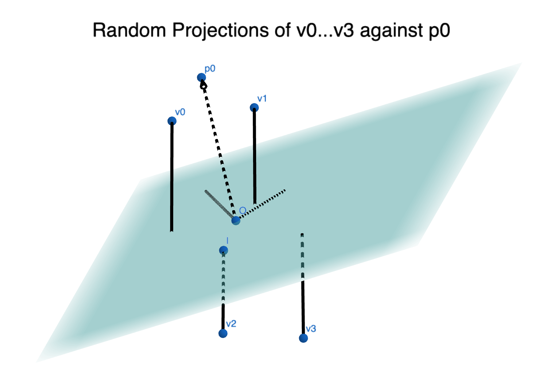
We can repeat this for many projections p0…p63, and get a 64 bit vector that represents v0 and v1 relative to those projections:

v0: 10111...001
v1: 10101...101
v2: 01001...010
v3: 00111...001

Now we know your work colleague is not only east of mississippi, but south of the Ohio, north of the Tennessee-Kentucky border, etc etc… How many of those properties you share with your coworker may dictate whether you can grab a coffee or not at your next 1-1.

v0:        10111...001
v1:        10101...101
...
v10000:    11110...100

So now we have compressed the 10000 vectors to: 10000 64 bit integers plus 64 projections. If each vector is a float32, that’s

• Uncompressed bits: 10000 * 32 = 320000 bits
• Compressed bits: 64 * 32 + 10000 = 12048 bits

A pretty massive space savings. We can index far more vectors than what we have in memory.

Hamming similarity – how do we recover the similarity

At search time, you can approximate the dot product, between v0 and v1, you simply count how many bits overlap, and divide by number of bits.

If we have 8 bits:

v0:        10111001
v1:        10101101

v0 and v1 share 6 bits out of 8, or have a hamming similarity of 0.75. That means 75% of the time they land in the same “side” of random hyperplanes.

Given those same 64 projections, we could compress thousands of vectors into just 64 bits:

Your work colleague is east of mississippi, south of the Ohio, north of the Tennessee-Kentucky border… and you’re ALSO east of mississippi, south of the Ohio, north of the Tennessee-Kentucky border… You might be able to meetup for coffee!

The more hyperplanes we use, the more accurate this will be at the cost of using more memory.

Implementation - pure python numpy

It’s relatively easy if you know a little numpy to implement random projections. My repo of numpy similarities has code you can follow along.

First, we build a random projection rather simply:

def random_projection(dims):
    """Sample a unit vector from a sphere in N dimensions.

    It's actually important this is gaussian
    https://stackoverflow.com/questions/59954810/generate-random-points-on-10-dimensional-unit-sphere

    IE Don't do this
        projection = np.random.random_sample(size=num_dims)
        projection /= np.linalg.norm(projection)

    """
    projection = np.random.normal(size=dims)
    projection /= np.linalg.norm(projection)
    return projection

Importantly, because we need evenly distributed projections around a normalized sphere, we nee to sample from a normal distribution.

We stack up however many projections we want:

def create_projections(num_projections=0,
                       dims=0) -> np.ndarray:
    """Create a set of random projections."""
    projs = []
    for _ in range(num_projections):
        projs.append(random_projection(dims))

    return np.array(projs)

Then given a vector, to index the rows, all we have to do is set or clear bits according to the projection:

def index(vectors, projections):
    if len(projections) % 64 != 0:
        raise ValueError("Projections must be a multiple of 64")
    hashes = np.zeros((len(vectors), (len(projections) // 64)), dtype=np.uint64)
    for vect_idx, vect in enumerate(vectors):
        for bit_idx, proj in enumerate(projections):
            dot = np.dot(vect, proj)
            if dot >= 0:
                hashes[vect_idx] = set_bit(hashes[vect_idx], bit_idx)
            else:
                hashes[vect_idx] = clear_bit(hashes[vect_idx], bit_idx)
    return hashes

(You can look at the bit twiddling code in the repo that sets, clears, and counts the bits)

Search time, given vector q, just means creating a hash for q – by running it through the same projections – and then doing hamming distance on it.

q:  10111...1101
v0: 10110...1010

To count shared bits we first XOR q and v0, to get all the dissimilar bits

q:   10111...1101
v0:  10110...1010
XOR: 00001...0111

We could actually compute the shared bits by bitwise inverting XOR now:

q:    10111...1101
v0:   10110...1010
XOR:  00001...0111
~XOR: 11110...1000

But there’s not much point in getting the true number of shared bits. We know XOR is the inverse and thus an XOR closer to 0 set bits is more similar.

def hamming_naive(hashes, query, count_function=bit_count64):
    """Row-wise compute hamming distance of hashes relative to query."""
    return np.sum(count_function(hashes ^ query), axis=1)      # Count bits in the XOR

(bit_count64 here is just bit twiddling to count the number of bits)

Putting all the pieces together, you can see the full query function:

def query_pure_python(vector, hashes, projections, hamming_func=hamming_naive, n=10):
    # Compute the hashes for the vector
    query_hash = index([vector], projections)[0]

    # Compute the hamming distance between the query and all hashes
    hammings = hamming_func(hashes, query_hash)

    # Sort ascending, 0 is most similar
    idxs = np.argsort(hammings)[:n]
    lsh_sims = hammings[idxs]
    return idxs, lsh_sims

This function returns the ids of the similar rows, ‘idx’ and also the similarities themselves, lsh_sims.

How good bad is it?

You can benchmark using the glove 600B token, 300 dimension dataset with the script in the repo:

# Arguments <implementation> <projections...>
python benchmark/glove.py pure_python 64 128 256 512 1280

To say the query latency is terrible… is an understatement 😎.

We have from tens to low single digit QPS😱. We get recall ranging from 0.1 to 0.56. As a comparison hnswlib on the same hardware gives in the 100-1000s of QPS with the best latency here (0.56). Recall even closer to 0.9 with the same latency (much lower at reasonable latencies).

64 projections -- QPS 15.287508822856918 -- Recall 0.14599999999999982
128 projections -- QPS 9.070002972455834 -- Recall 0.16499999999999987
256 projections -- QPS 6.6515773960504685 -- Recall 0.20699999999999996
512 projections -- QPS 4.8655798116102 -- Recall 0.3990000000000001
1280 projections -- QPS 2.573814908986091 -- Recall 0.5639999999999997

As a graph:

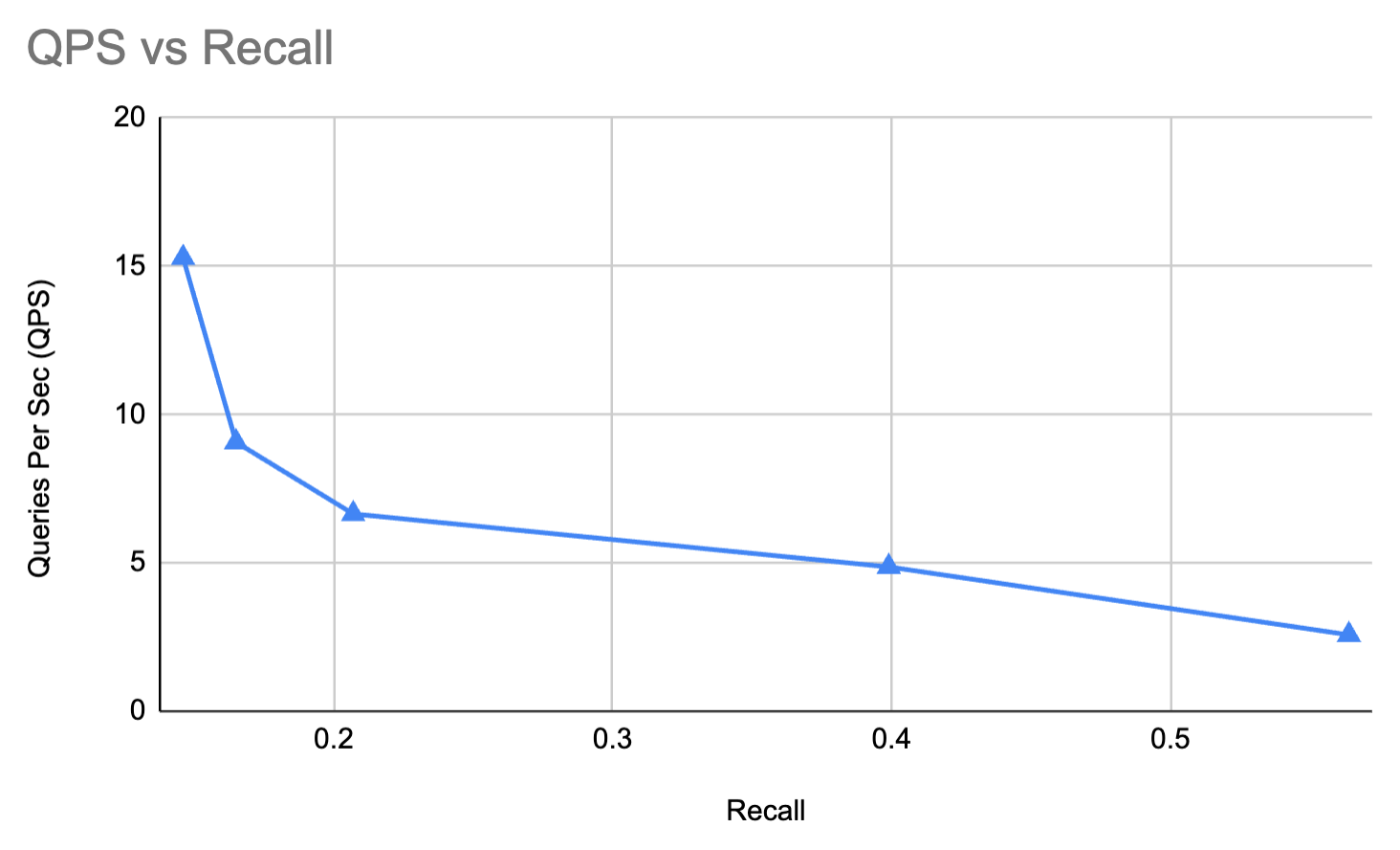
Query latency wise, it’s worse than bruteforce. And let me sell it to you further: it gets terrible recall. As you’d expect, recall goes up with number of projections. Query latency goes down. Not surprising.

But that’s not where the concerns begin: Some are simply foundational in this algorithm.

Lesson 1: recovering similarities != nearest neighbor search

It can’t be stated enough LSH approximates similarities, not neighbors.

That’s a subtle difference, but an important one. Knowing how close two points are is NOT the same as knowing whether they’re neighbors.

Think about the distribution of people on the surface of the Earth.

Some people cluster very closely. A small error in the location of a New Yorker would put them a “block” away from their actual location, giving them very different neighbors. If you want to find a “nearby” coffee shop in New York City, the notion of “nearby” is probably very very close, like 0.1 km. Screwing that up, even a little bit, teleports you to a completely different neighborhood of the city.

This wouldn’t be a problem in the middle of a rural Kansas. You could screw up the user’s location A LOT. Several 10s of kms, and you’d still suggest the closest coffee shops. Recovering a notion of “similarity” between coffee shop and user would likely be sufficient.

Most embeddings lump together. Some regions get VERY busy - like an ant colony of semantic meaning - others have vast stretches of vacuum.

Further it’s not evenly distributed per dimension. Simply look at our Earth again. We mostly think in two dimensions. We rarely think of distance in terms of a 3rd dimension: altitude. But its there!

This is why graph algorithms like HNSW perform so well on nearest-neighbors benchmarks. They actually map out an actual network of neighbors, directly solving for recall in nearest-neighbors problem. Much like how zip codes or area codes can be very small in dense places and very large in others.

Lesson 2: LSH must scan the hashes

Naive, simple, LSH must scan the hashes to recompute similarities. Unspurprisingly, this will be a natural limit to the speed of this algorithm. Not much else to say about this.

Lesson 3: Python -> C roundtrips slow us down.

While numpy itself is fast, when you profile the code, you see discrete steps in the query function that dominate the runtime:

         258304 function calls in 39.622 seconds

   Ordered by: cumulative time
   List reduced from 27 to 20 due to restriction <20>

   ncalls  tottime  percall  cumtime  percall filename:lineno(function)
      100    0.002    0.000   39.619    0.396 lsh.py:76(query_pure_python)
      100    4.552    0.046   31.425    0.314 hamming.py:41(hamming_naive)
      100   25.139    0.251   25.139    0.251 hamming.py:21(bit_count64)
      100    0.000    0.000    7.928    0.079 fromnumeric.py:1025(argsort)
      100    0.000    0.000    7.928    0.079 fromnumeric.py:53(_wrapfunc)
      100    7.927    0.079    7.927    0.079 {method 'argsort' of 'numpy.ndarray' objects}
      100    0.001    0.000    1.735    0.017 fromnumeric.py:2177(sum)
      100    0.001    0.000    1.734    0.017 fromnumeric.py:71(_wrapreduction)

• Each call within hamming itself, such as x’oring two arrays, then bit twiddling with numpy, is a roundtrip from Python to Numpy’s C code for these operations.
• Argsort itself to get the bottom N hamming similarities is a pretty hefty operation here

So an obvious step is to not have a “pure_python” implementation, and move as much functionality into numpy C code that can directly process the array. Still limited by the above two factors (similarity != nearest neighbors; needing to scan). We’re unlikely to squeeze extra recall, but we could probably increase QPS several orders of magnitude.

We’re also using only one CPU here, and one wonders if you can speed things up further by splitting out these operations over many cores.

And finally, there ARE other classing LSH algorithms like spectral hashing that would be fun to learn.

Arguments FOR hashing functions in nearest neighbors search

At a previous job as a performance oriented C-developer, we had a phrase that “O(n) often beats O(log(n))”. (I believe this is from Raymond Chen, but I can’t find the original quote.)

Why is that?

Well mostly cache locality. Juggling data structures that contain lots of pointers, pointing to many different regions of memory, jumping around tends to hurt performance. Code complexity matters to. A dumb array with simple looping operations can be easier to optimize, with few variables, and it’s usually easier to build and maintain anyway.

One reason I keep going back to this hashing well is because is there’s also just the epic simplicity here around common search operations:

• Adding a new vector to this “database” just appends to the hashes
• You can segment/shard these all you want to colocate documents with other stores
• You can freeze them and parallelize the search of the hash array

Graph solutions are big global data structures “things with pointers”. HNSW hasn’t worked well for Lucene exactly for this reason, it doesn’t fit into its more segmented and sharded operational model. A global “graph” resists being broken up and sharded. Though Vespa appears to have found an interesting approach.

So operationally, this sort of thing seems like it could be a winner. I know exactly what problems I’ll run into (New Yorker / ant colony problems). But with good-enough latency, it might be OK. And besides, embedding similarity is just one of many other factors to consider with search ranking. And ranking itself, is just one factor among many things that dictate search quality.

Feedback welcome

In future posts, for my own edification, I’ll hopefully teach you how to hook up ANN Benchmarks to your own algorithm. I’ll also dig into the C implementation that, spoiler alert, gives much better QPS for… the same recall :). At least enough to serve as research a baseline for others who are building ANN.

I hope you share feedback either directly or through social media!