Expanding on my Cheat at Search Essentials training class, I decided to go beyond just plain-old-BM25, to multi-field BM25, or BM25F.
Search engines like Elasticsearch use BM25 to rank search results. BM25 answers an important question — IF we see a query term match, how much is that passage about the matched term? That’s not all of what search relevance is, but it’s an important part. This question underlies not just BM25, but emerging sparse models (which themselves might need to retrieve across fields!).
Get to know the BM25 building blocks
Numerous articles go into great depth on BM25 and why its the golden baseline for search. But I’ll work to capture the building blocks a bit differently. We’ll take these pieces and use them to build BM25 for multiple fields.
First realize most search systems, for years, scored results using three primary inputs:
| Factor | Definition | Impact to score |
|---|---|---|
| Term Frequency | a word count, how often does skywalker occur in this document? |
Higher (more frequent) is good! |
| Document Frequency | rareness, if searching for luke OR skywalker , luke is common/ambiguous while skywalker is rare/specific. |
Lower (more specific) is good! |
| Field Length | number of terms in a field (matches or otherwise). | Matches on shorter fields seen as more important than longer |
We get the name TF*IDF from TF / DF from these stats.
Throughout history, we have learned how to best use these ingredient; lessons now baked into BM25. Lessons that came from countless studies, across numerous domains, of how users view the relevance of term matches.
Getting these basics down, we’ll then see how we mix them together to go beyond a single field, to build up BM25F with multiple fields.
BM25’s Document frequency
First, we know a bit how users perceive a terms specificity. We usually say a term that rare in the corpus is more specific to the users intent. A rare terms occurrence in an irrelevant document is less probable than a common one.
We’ve learned users notion of specificity isn’t linear. A term occurring in 2x fewer docs is not 2x closer to the users intent.
Notice below, in BM25’s IDF scoring, for every 100 raw document frequency, we don’t get a linear decrease in specificity. At first the drop off is steep. Then it tapers.
BM25 decays specificity logarithmically, IE this formula seems to work best:
def compute_idf(num_docs, df):
    """Calculate idf score from num_docs (index size) and df (a term's doc freq)"""
    return np.log(1 + (num_docs - df + 0.5) / (df + 0.5))
When we get to multiple fields, we’ll need to account for every fields differing document frequency stats. More on that below.
Scaling term frequency to document length
Pickup a copy of Proust’s In Search of Lost Time and you’ll have to read maybe a million words? Read a tweet, you’ll encounter maybe a dozen?
If Proust happened to use the term skywalker it’d be pretty weird. But maybe not entirely unexpected to happen accidentally once in 4000 pages. A term frequency of “1” in Proust should be seen as low-information relative to the term occurring a thousand times. We would not say the book is “about” skywalker or Star Wars by one mention.
If a tweet mentions skywalker once, wow, that one occurrence is very important to the tweet! It’s like 10% of the information! The tweet is very much about skywalker
BM25 scales term frequency so that long document’s TF counts less than short documents:
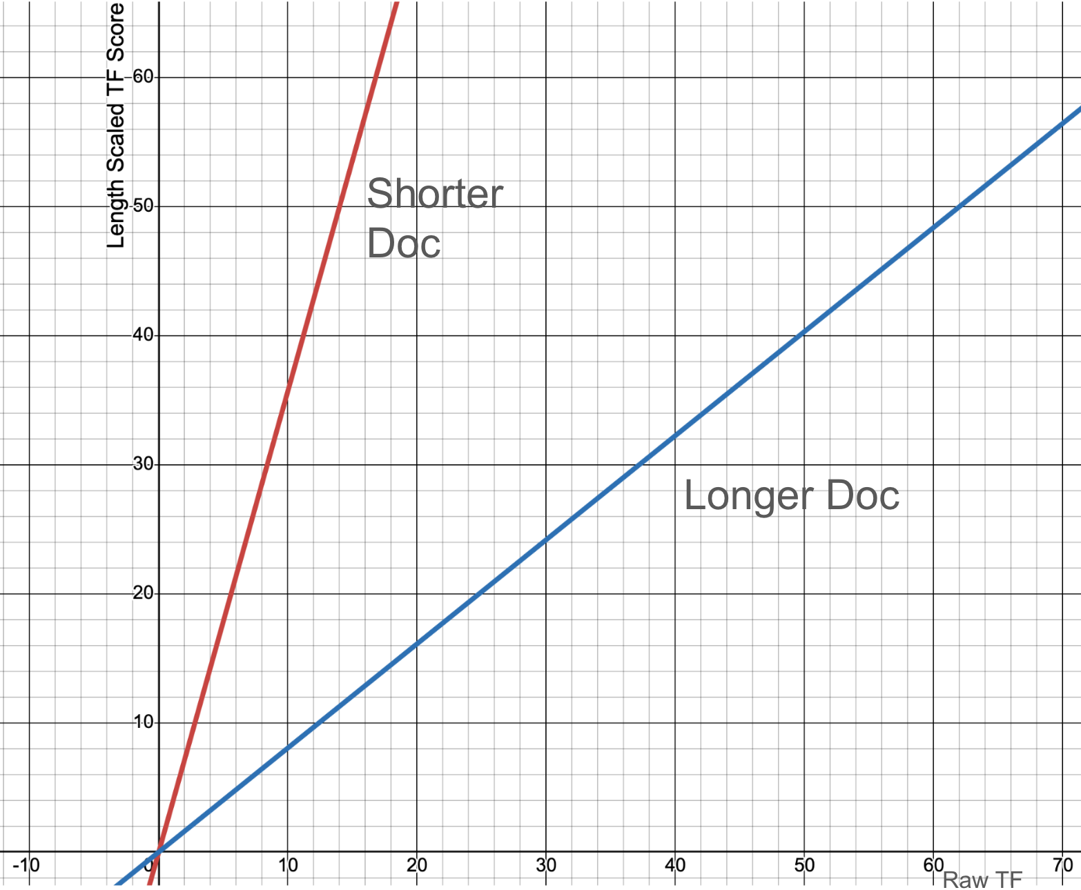
It’s a simple formula, with parameter b that changes how much document length influences the term freq score:
def scaled_tf(term_freq, doc_len, avg_doc_len, b=0.8):
	(term_freq) / (1 - b + b * doc_len / avg_doc_len)
With multiple fields, each field has a different length. We’ll have to account for each filelds length independently.
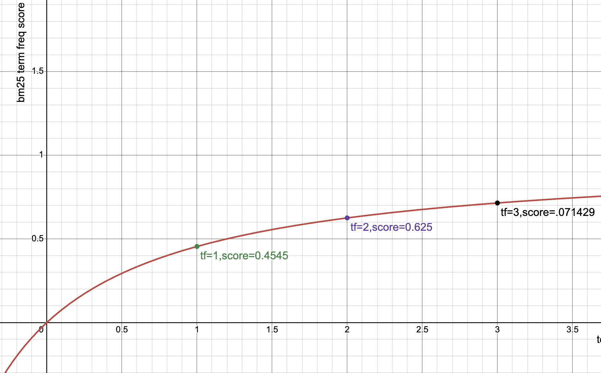
Term frequency saturation
As a passage mentions a term more-and-more times, users don’t think its relevance goes higher and higher, it plateaus.
You’re reading a blog post, you see the word bm25 mentioned. Oh wow maybe this article is about bm25? You see it a second time - confirming your suspicions. Then a third, fourth, fifth, … 99th time. By the 99th time you see bm25 in the article, it can’t get much more relevant to the term. We get it by now.
Information Retrieval experiments confirm, relevance perceptions reach of point of saturation after they’ve seen a term enough. In other words, like document frequency, term frequency starts off strong with each incremental mention of a term, but gradually peters out.
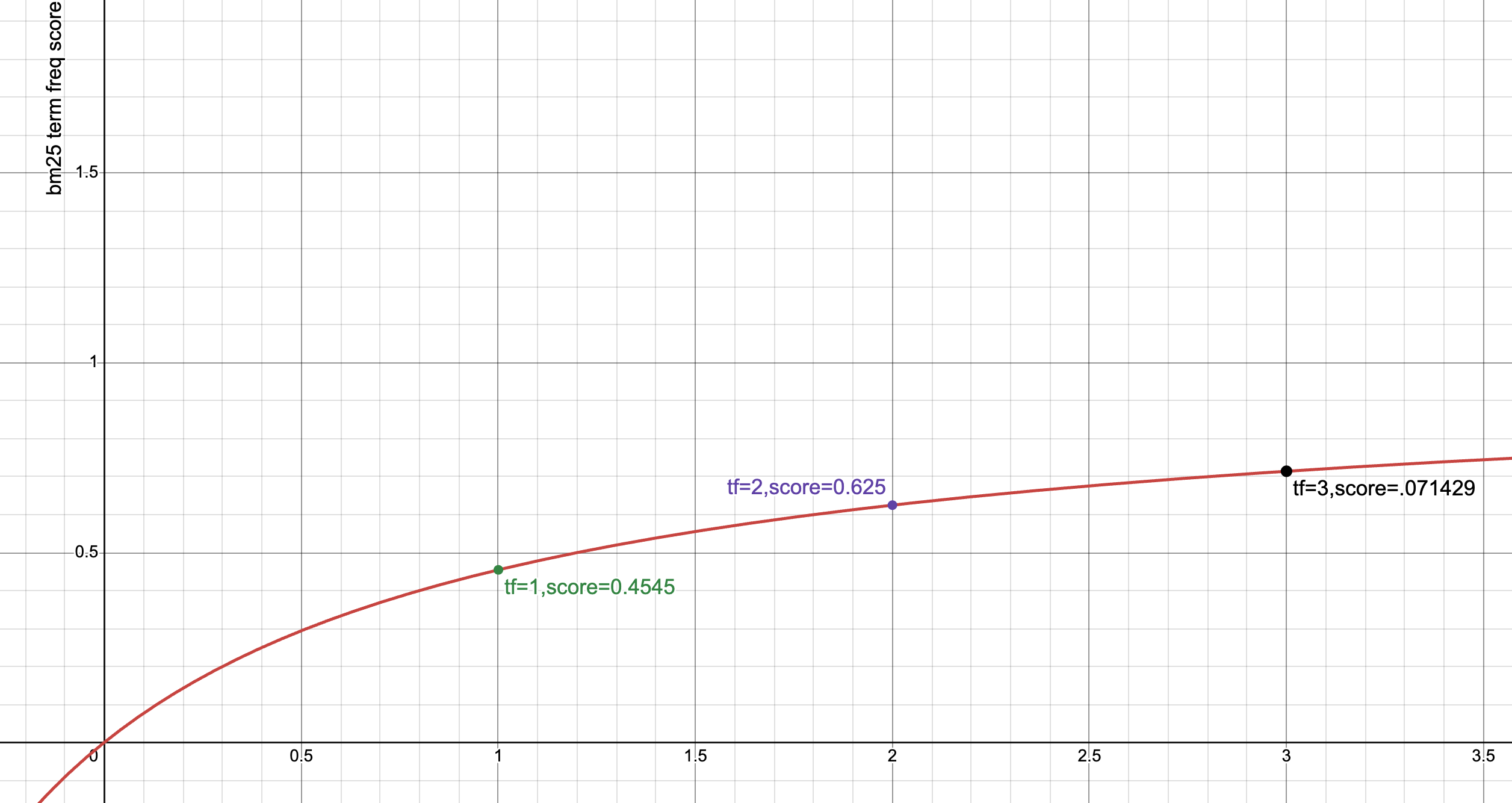
The math for this is simple, with a constant k1 controlling the rate of saturation:
def bm25_tf(termfreq, k1=1.2):
	return termfreq / (termfreq + k1)
(Note I’m using the Lucene formulation which removes the k1 + 1 in the numerator for performance as it doesn’t impact ordering)
BM25 put together
Now we need to compute TF * IDF but BM25 style, by putting together everything from below.
IDF we can just take from above.
But the “TF” part we combine the scaled_tf and the bm25_tf , giving the classic BM25 TF formula:
def bm25_scaled_tf(term_freq, doc_len, avg_doc_len, b=0.8):
	(term_freq) / (termfreq + k1 * (1 - b + b * doc_len / avg_doc_len))
The math here saturates with a tf / (tf + constant). That constant is tuned to the document length (it’s the bit that bends the line above). But instead of bending a line, we’re bending the saturation curve.
Multifield TF*IDF requires us to derive a kind of TF and a kind of IDF for a term across multiple fields. First we will start with IDF.
BM25 Problems with fielded search - specificity
Almost all full-text search engines break the index into mini-indices we search called fields. Like for books maybe title, body, or description. Each field lives in its own universe of scoring statistics (average document length, term and document frequencies, etc).
It turns out, raw BM25 has a few problems when text is split across fields.
In a technical book search I worked on, some book publishers would put “book” in the title. It wasn’t common. But try to imagine what BM25 would do when a user searched for javascript book . Thousands of technical books have javascript in the title. A few, spurious books have book in the title.
Because books high IDF, you’d get weird results with no Javascript! Such as:
Query: Javascript Book
- The big book on squirrels
- C Programmers Book about Pointers
- The missing iPhone book
The root of the problem: document frequency of book in the title field doesn’t reflect its actual specificity in the full corpus. If we looked at other fields like body and description we might (though still not fullproof!) get a better sense of book’s specificity.
This is the first spot where BM25F comes to help. If we were to naively sum BM25 scores across fields, we would end up with the busted results above, strongly biased towards the rare title matches.
score = TF('title', 'book') * IDF('title', 'book') \
        + TF('body', 'book') * IDF('body', 'book')
A better way to model specificity, would be to somehow know the true document frequency across fields, then compute IDF score using that. Usually, this is done by simply taking the max document frequency.
combined_doc_freq = max(DF('title', 'book'), DF('body', 'book'))
blended_idf = compute_idf( corpus_len, combined_doc_freq)
Elasticsearch has a query mode called cross_fields . It does just this combining part. Elasticsearch cross_fields blends document frequencies, then repeats the math from above:
score = TF('title', 'book') * blended_idf \
        + TF('body', 'book') * blended_idf
It’s a good-enough 80% solution that captures the biggest problem with BM25 across fields. But it’s not all the way to BM25F.
Multi field TF double counts
Another problem with naive BM25 summing occurs with the combination of term frequencies. If we just blend document frequencies, but leave term frequencies alone, we let each term saturate independently.
score = TF('title', 'book') * blended_idf \
        + TF('body', 'book') * blended_idf
Here we might see title:book match once, and count it very strongly (it’s early in the saturation curve). While body:book is mentioned hundreds of times, but we also count its early trips in the saturation curve.
| Match of body | Impact | Notes |
|---|---|---|
| Title (tf=1) | High | Early in saturation curve |
| Body (tf=100) | High but diminishing | Farther in saturation curve |
| Total | 2 x High + diminishing | double counted |
In reality what we want to see is something like
| Match of body | Impact | Notes |
|---|---|---|
| Title + Body (tf=101) | High but diminishing | |
| Total | High but diminishing |
BUT and this is a big but 🍑
Comparing these term frequencies is like an apples to oranges comparison. Remember how document length modulates term frequency. The 1 term freq in short title should count much more than the 100 terms in the body. Maybe we’d say that title term freq should be scaled up. While the body scaled down.
So looking at a length-normalized situation, what we’d actually want is maybe the following (with fake, hand waving scaling up/down)
| Match of body | Impact | Notes |
|---|---|---|
| Title (tf 1 → 5) + Body (tf=101 → 30) | High but diminishing | |
| Total: 35 | High but diminishing |
So that’s where we apply these steps
- The length normalization step to scale up / down each field’s term freq →
scaled_tffrom above - Apply saturation to the output of this (
bm25_tf)
The final combined “TF” becomes:
bm25_tf(scaled_tf(TF('title', 'book'), title_len, avg_title_len) +
        scaled_tf(TF('body', 'book'), body_len, avg_body_len))
So the final BM25F looks like:
combined_doc_freq = max(DF('title', 'book'), DF('body', 'book'))
blended_idf = compute_idf( corpus_len, combined_doc_freq)

bm25f_tf = bm25_tf(scaled_tf(TF('title', 'book'), title_len, avg_title_len) +
                   scaled_tf(TF('body', 'book'), body_len, avg_body_len))


bm25f = blended_idf * bm25f_tf
And that’s it, now you know BM25F, and maybe even have a deeper intuition about BM25 itself!
What questions do you have about sparse document scoring? How would we do a multi-field search for a sparse transformer model? Is document frequency the only / best way to compute term specificity? How do we extract our tokens from the raw strings? Tokenization is another important design point in a lexical system to accurately reflect when a ‘match’ truly occurs.
A lot of open questions still and room for you to innovate and tune in lexical. Get in touch if you’d like to chat more!
Enjoy softwaredoug in training course form!
Starting May 18!
Signup here - http://maven.com/softwaredoug/cheat-at-search I hope you join me at Cheat at Search with Agents to learn use agents in search. build better RAG and use LLMs in query understanding.

Doug Turnbull
More from DougTwitter | LinkedIn | Newsletter | Bsky