Across several search jobs, a simple question has dominated product discussions
What search queries could be performing better? A simple question. But its more complicated than you might appreciate.
The finer you slice, smaller the sample, the higher the noise.
Ever seen an election poll? This poll says Trump is ahead of Harris 2%. But some Harris supporter goes and looks at the crosstabs: well female voters from Georgia, actually are surging for Harris! The election is in the bag!
The problem is there are 5 individuals polled that meet this description. It’s almost certain at such a small sample size, you can’t draw much of a conclusion about the overall population. You must avoid getting lost in the crosstabs.
Thus is the problem too. You want to take your A/B test success metric (Add to carts up 2% in test vs control!) and then look at individual search queries – why are queries for “red high heel shoes for squirells” down 50%!?!? Of course this query happened TWICE in one month.
Slicing down to tiny sample sizes means… you’re just getting more and more noise. Even slicing down to seemingly mundane, frequent queries can show this problem. Almost no correlation between individual query performance and outcomes. It’s all noise!
Ugh…
Yet we MUST have query level data to debug our system. We need a sense of which types of queries perform well and which perform poorly. Otherwise we have no basis for our future improvements. We’re up 💩 creek without a paddle. 🛶.
What we want to answer: if we slice a metric down to a query, can we trust the conclusion? We need two things:
- Is the query’s performance relative to the average query performance statistically significant?
- Is that statistical significance trustworthy - ie does it have statistical power
Global rate vs local rate
Statistical significance is simple enough. We have a metric, let’s say Add-to-carts. We know an average query has 0.05 add to carts.
Then we have our query:
| Avg Query (global) | Query: ‘red shoes’ (local) | |
|---|---|---|
| Add-to-carts | 50,000,000 | 2 |
| Num Sessions (n) | 1,000,000,000 | 100 |
| Add-to-cart rate | 0.05 | 0.02 |
Our null hypothesis is “there is no difference” between the add-to-cart rate of “red shoes” and the global add-to-cart. Red shoes is not any better/worse.
How can we test this hypothesis?
Add to cart rate compares two proportions. We can “pool” the proportions here (the add to cart rate) into a pretend, combined ATC rate. This lets the red-shoes query tug the global one way or another. The pooled proportion is:
Pooled Proportion = (ATC global + ATC local) / (Num Sessions global + num sessions local)
We won’t tug this very far in this case:
Pooled Proportion = (50000000 + 2) / (1e9 + 100) = 0.49999997
Even though its a tiny difference, we have to ask, how far is it from the expected mean of the difference? We would need to know the std deviation of Global Distribution minus Local distribution. We can get that by taking the standard error of the difference, which estimates the standard deviation:
Std Error = SQRT(Pooled Proportion * (1 - Pooled Proportion) * (1 / n_global + 1/n_local)
In our case:
Std Error = SQRT(0.49999997 * (1 - 0.49999997) * (1 / 1e9 + 1/100)) = ~0.05
If std error is the std deviation from the difference, we can ask, how far (in units of std deviations) is our Add To Cart rate from the expected mean of a difference of 0? We call this the z-score:
z_score = (local_ctr - global_ctr) / std_error = (0.02 - 0.05) / 0.05 = -0.6
And if we assume the difference is normally distributed, we can find -0.6 on the x-axis in the probability distribution, the colored in area indicates the probability we can reject the NULL hypothesis.

We can compute this with the CDF function which takes the z-score (std devs from mean) and returns the probability.
In this case, it’s hard to definitiely reject the Null hypothesis, the probability of red shoes having this add to cart rate when no difference should exist between this query and the gloabal is p=0.274.
A more common query
Let’s rerun our significance test, but for a more common query. We find plain jane shoes occurrs more frequently, but a similar ATC rate as red shoes:
| Avg Query (global) | Query: ‘shoes’ (local) | |
|---|---|---|
| Add-to-carts | 50,000,000 | 20 |
| Num Sessions (n) | 1,000,000,000 | 1000 |
| Add-to-cart rate | 0.05 | 0.02 |
Running through our calculations again
Pooled Proportion = (50000000 + 20) / (1e9 + 1000) = 0.049999997
Std Error = SQRT(0.049999997 * (1 - 0.049999997) * (1 / 1e9 + 1/1000)) = ~0.00689
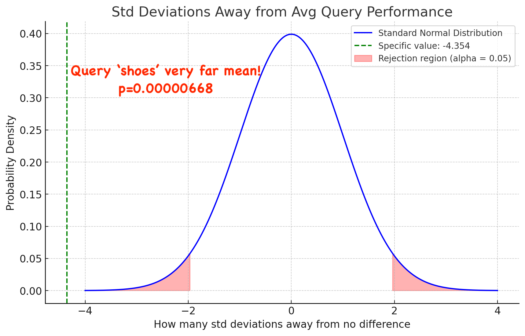
z_score = (0.02 - 0.05) / 0.00689 = -4.354
So approximately -4.354 std deviations below the expected mean (p=0.000000668!)
A note on statistical power
You see that when we increase the number of observations in our query, the pooled-propotion pulls farther from the mean, and the std error / deviation of the difference decreases. This makes it easier to detect an effect.
So generally, it would be difficult to have a false positive. The opposite is not true. We COULD have an effect, but we lack sufficient statistical power to know. AKA a Type 2 error.
We can try to measure this by choosing a z-score (let’s say 1.9599, which corresponds to p=0.05) and seeing how likely our z-score would avoid a false negative, if the test showed a negative:
Power = 1 - NORMDIST(0.6 - 1.9599,0, 1, TRUE) + NORMDIST(-0.6 - 1.9599, 0, 1, TRUE)
Here power is ~0.092 so about a 9.2% chance a negative is a false negative.
Generally, because the pooled proportion increases our confidence, we can simply rely on increased significance being the result of large delta AND a large population of queries (such as shown above)
Please criticise this!
I blog to get less dumb. What gaps do I have in my understanding of comparing two proportions?
I still have some confusions:
- Why do we assume a std deviation of 1 in the power test?
- Is it safe to assume that the role of power primarilly is to measure likelihood of false negatives? And that you wouldn’t get “underpowered false positives” in this approach?
- It’s assumed, by the central limit theorem, that the difference between the distributions is normal. Is that an appropriate assumption when queries are likely to follow a strong power law distribution?
I hope this article is useful, and as always, thanks for letting me know anything I missed :)
Upcoming course: Build your own vector database

Want to understand what makes embedding retrieval fast, relevant, and useful in real AI systems? Join Build your own vector database and build the core pieces yourself, from embeddings and indexing to search and retrieval.

Doug Turnbull
More from DougTwitter | LinkedIn | Newsletter | Bsky