A Roaringish phrase search algorithm

SearchArray adds boring, old BM25 full text search to the PyData stack.

A full-text search index comes with one underaprreciated problem: phrase search. In this article, I want to recap a roaringish phrase search algorithm, encoding positions in a roaring-like numpy array for fast bit intersections.

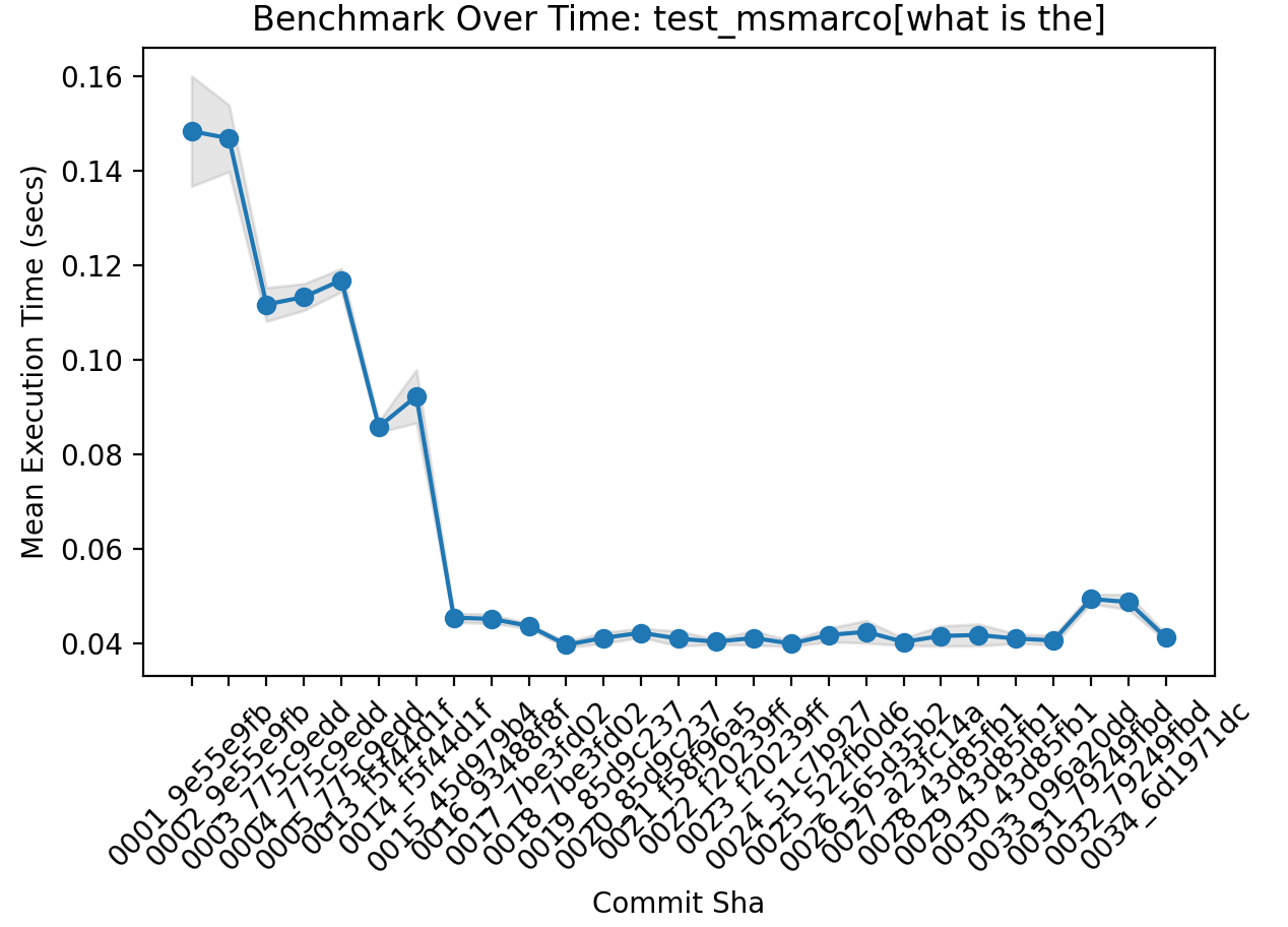
But before such magic, I’m ashamed to say, SearchArray started with very primitive approaches. SearchArray took almost 5 minutes(!!) for a phrase search to complete on 100k MSMarco docs. Luckily now I’ve gotten those numbers down quite a bit:

SearchArray refresher

Let’s remember how SearchArray works. It’s built as a Pandas extension array that represents an inverted index, demoed below.

In [1]: import pandas as pd
        from searcharray import SearchArray

In [2]: df = pd.DataFrame({"text": ["mary had a little lamb the lamb ate mary",
   ...:                             "uhoh little mary dont eat the lamb it will get revenge",
   ...:                             "the cute little lamb ran past the little lazy sheep",
   ...:                             "little mary ate mutton then ran to the barn yard"]})

In [3]: df['text_indexed'] = SearchArray.index(df['text'])

In [4]: df
Out[4]: 
                                                text                                       text_indexed
0           mary had a little lamb the lamb ate mary  Terms({'little', 'mary', 'a', 'lamb', 'had', '...
1  uhoh little mary dont eat the lamb it will get...  Terms({'eat', 'it', 'will', 'little', 'revenge...
2  the cute little lamb ran past the little lazy ...  Terms({'little', 'sheep', 'lazy', 'cute', 'lam...
3   little mary ate mutton then ran to the barn yard  Terms({'barn', 'little', 'mary', 'mutton', 'ya...

Now we can get a BM25 score for each row of text_indexed, looking for the phrase “little lamb”:

In [7]: df['text_indexed'].array.score(["little", "lamb"])
Out[7]: array([0.19216356, -0.        , 0.18430232, -0.        ])

Under the hood of text_indexed, we’ve got an inverted index that looks like:

mary:
   docs:
     - 0:
         posns: [0, 8]
     - 1:
         posns: [2]
little:
   docs:
     - 0:
         posns: [3]
     - 1:
         posns: [1]
     - 2:
         posns: [2, 7]
     - 3:
         posns: [0]

lamb:
   docs:
     - 0:
         posns: [4, 6]
     - 1:
         posns: [6]
     - 2:
         posns: [3] 

If a user searches text_indexed for like lamb, we can recover its term frequencies (doc 0 has 2 occurences, doc 1, 2, etc), document frequency (lamb occurs in 3 docs), everything we need for a BM25 score.

But what about phrase search? How do we compute not just term frequencies, but phrase frequencies?

How would we count all the places where “little” comes one position before “lamb”?Looking at doc 2 above - if little occurs at positions [2, 7] (2nd and 7th location) and lamb at position [3], how do we detect that lamb’s has one case of occuring exactly one location after little?

Bigram by bigram search

To implement phrase search, we connect the dots, one bigram at a time.

If a user searches for “mary had a little lamb” we first connect mary -> had. We then then repeat the process, except now we find where mary+had bigram positions occur immediately before a’s. If mary+had bigram ends at positions [1, 6] in a document, and that document has an a at position [2], then now mary+had+a trigram occurs ending at position [2].

Now we continue to finding the quadram mary+had+a+little. Maybe little occurs at position [3] in this doc. Now we have narrowed to a quadgram at mary+had+a+little ending at [3].

Now we connect mary+had+a+little positions to lamb, getting to the end of our phrase.

The number of times mary+had+a+little occurs before lamb is our phrase frequency.

It’s this connecting detail that concerns us. How do we find where one set of position occurs immediately before another set of position (ie mary before had, etc)? How do we do this fast enough to make SearchArray usable?

From Boring to Roaring

Let’s dig into how to intersect two sets of positions.

Early, naive versions of SearchArray, stored each doc/terms position integers directly as raw integer arrays. I had many different ways of finding bigram adjacencies - from subtracting one terms positions from another to intersecting the positions.

Storing the integers directly takes up way too much memory. For a meaty search dataset, storing giant positional arrays, per term, is simply a non starter to do meaningful work.

Time to rethink things.

I knew a bit about roaring bitmaps. Roaring bitmaps store sets of integers as bitmaps. I won’t take you through a tutorial of roaring bitmaps themselves. What I did was roaring-adjacent, or roaringish. Let’s walk through that.

The main intuition I took from roaring bitmaps was the following: follow along in this notebook

Let’s say we want to pack positions into a 32 bit array. Looking just at one term, we have

import numpy as np

posns = np.array([1, 5, 20, 21, 31, 100, 340], dtype=np.uint32)
groups = posns // 16
values = (posns % 16)

groups, values

Output:

(array([ 0,  0,  1,  1,  1,  6, 21], dtype=uint32),
 array([ 1,  5,  4,  5, 15,  4,  4], dtype=uint32))

By dividing by 16 (groups), and modulo by 16 (values), we’ve segmented up the positions into groups. Let’s zoom in group-by-group:

Positions grouped by posn // 16:
-------------------------
        Group 0: | Group 1:  | Group 6: | Group 21:
values: 1, 5     | 4, 5, 15  | 4        |   4

We can bitwise OR each groups values together into 16 bit values per group:

Group 0             Group 1            ...       Group 21
0000000000100010    1000000000110000   ...       0000000000010000
(bits 1 and 5 set)  (bits 4, 5, 15 set)          (bit 4 set)

Moving now to a 32 bit value, we can store the group number in the upper 16 bits:

Group 0                              | Group 1                             ...      | Group 21
0000000000000000 0000000000100010    | 0000000000000001 1000000000110000   ...      | 0000000000010101 0000000000010000
(group 0)        (bits 1 and 5 set)  | (group 1)        (bits 4, 5, 15 set)  ...    | (group 21)       (bit 4 set)

We can do this in numpy, pretty easily, continuing the code from above:

# Find the boundaries between MSB groups
change_indices = np.nonzero(np.diff(groups))
change_indices = np.insert(change_indices, 0, 0)

# Set 'values' bit
values = (1 << values)

# Pack into 7 32 bit integers
packed = (groups << 16) | values

# Combine into groups by oring at specific index boundaries
packed = np.bitwise_or.reduceat(packed, change_indices)

The key here is doing a bitwise_or, but over a specific set of indices change_indices. This packs only where the MSBs differ, at their boundary.

And now… 7 original positions are now packed into 4 32 bit values. Shrinkage!

Finding bigrams through bitwise intersection

Now, given two sets of term posns, we might find their bigram frequency by simple bit arithmetic.

Given two sets of positions for little and lamb

1. Intersect the two term’s MSBs (ie the 16 MSBs)
2. Shift the left term’s lower 16 LSBs (the posns) to the right by 1
3. Bitwise AND the LSB’s
4. Count the number of set bits in the 16 LSB == phrase match!

Walking through an example:

Say we have term “little”, with positions encoded

Group 0                              ...    | Group 21
0000000000000000 0000000000100010    ...    | 0001000000100101 0000000000010100

And given “lamb”

Group 1                              ...    | Group 21
0000000000000000 0000000000100010    ...    | 0000000000010101 0000000000101000

We note they share a “group 21” set of posns, corresponding to posns >= 336 but < 352 where adjacent positions might be found:

Group 21, little
0001000000100101 0000000000010100

Group 21, lamb
0000000000010101 0000000000101000

We now zero in on just the LSB, to see if any littles occur before lambs in group 21 (posns 336-352). We do that simply with bit twiddling:

(0000000000010100 << 1) & (0000000000101000) = 0000000000001000

(shift 1 to see if adjacent)                 = number of bits == num terms adjacent

Or one phrase match (one bit set).

All in numpy Python we can just do this:

# Find where common MSBs occur between terms
_, lamb_indices, little_indices = np.intersect1d(lamb >> 16, little >> 16, return_indices=True)

# Just the lower 16 where they intersect
lamb_intersect_lsb = (lamb[lamb_indices] & 0x0000FFFF)
little_intersect_lsb = (little[little_indices] & 0x0000FFFF)

# Find direct phrase match
(little_intersect_lsb << 1) & lamb_intersect_lsb

Counting the bits of each value in the output gives us the phrase frequency.

Wait there’s more! Also packing the doc id

Here’s where roaringish gets really fast.

So far we’ve looked at phrase search one document at a time. What if we could phrase match the entire corpus for two terms in a handful of numpy operations?

Indeed, we can do just that by just also packing the doc id… and just concatting every docs packed posns together.

# Using 64 bits, put doc id in upper 32
doc1_encoded = doc_1_id << 32 | packed_doc_1
doc2_encoded = doc_2_id << 32 | packed_doc_2

# For every doc with 'lamb' store all positions
term_posns["lamb"]  = np.concatenate([doc1_encoded, doc2_encoded])

Now the 48 MSB lets us intersect docs + bit group MSBs. At search time we do the exact same as before:

lamb = term_posns["lamb"]       # Every doc's posns for "lamb"
little = term_posns["little"]         # Every doc's posns for "little"

# Find where common MSBs _and documents_ occur between terms (doc ID AND bit groups)
_, lamb_indices, little_indices = np.intersect1d(lamb >> 16, little >> 16, return_indices=True)

# Get every doc's phrase match fol 'little lamb'
matches = (little_intersect_lsb << 1) & lamb_intersect_lsb

This now finds phrase matches over all documents for the two terms.

To count term matches by doc id, we just add a little step to count bits, then sum the phrase freq at the doc id boundary.

# Grab the intersected values so we can get doc ids (of either, they're identical)
intersections = lamb[lamb_indices]

# Demarcate the indices where doc ids differ
doc_id_change = np.argwhere(np.diff(intersections >> 32) != 0).flatten() + 1
doc_id_change = np.insert(doc_id_change, 0, 0)

# Sum set bits per doc id
counted_bits = bit_count64( (little_intersect_lsb << 1) & lamb_intersect_lsb )
phrase_freqs = np.add.reduceat(counted_bits, doc_id_change)

We’ve now got bigram phrase frequencies for “little->lamb”. If we had a trigram “little->lamb->tacos”, we’d now repeat the same algorithm, just with little+lamb posns -> taco.

Optimizations and annoying little issues

Our data, with doc ids in the MSB, can be stored sorted. Making intersections faster.

Numpy’s own intersect1d doesn’t particularly know about sorted data. Our data can be stored sorted (by doc id, then MSBs), theoretically making the intersection much faster. Luckily Frank Sauerburger has us covered with a handy sortednp library for intersections, merging, and other operations on sorted numpy arrays. Allowing us to find intersections with exponential search.

Another issue, of course: the algorithm I describe will miss out on phrase matches where the phrase matches straddle two MSB groups. IE:

“little” before “lamb” but across two MSB groups:

"little" group 21
0000000000010101 1000000000000000

                                          "lamb" group 22
                                           0000000000010110  000000000000001

This isn’t that hard to handle, we just need to create a second bit twiddling pass. Intersecting the first term with the second term’s group + 1, and looking for this exact situation.

Additionally, my bigram intersection above walked bigram by bigram mary -> mary+had etc. We might be smart and actually intersect the two rarest terms first. This dramatically limits the search space for the other bigrams. Maybe, for example, we note lamb and little are rarest. So we can intersect first those two terms, and limit the other intersections to a reasonable search space.

Finally this algorithm focuses on direct phrase matching. What do we do when a user asks for slop? As in, the user indicates that set of terms can be within N positions of a direct phrase match? “little bobby lamb” still matches “little” “lamb” with a slop of 1?. This algorithm doesn’t (yet) handle this case (and all the little edge cases :) ). That’s very much WIP.

Results

The speedup results from this were impressive. On 100K very text heavy MSMarco docs, I took searches on my local machine from some several seconds on a stopwordish search (what is the) to 10s of ms. The primary bottleneck now being the intersection (snp.intersect).

I can see now, the next step would be to optimize this layer. Sorted intersections on id sets can also be done with skiplists, which I believe is how most search engines implement this. But for now, this performance is good enough for my needs!

Additionally memory usage of 100K MSMarco docs shrunk by an order of magnitude. Making it closer to reasonable to do meaty, medium-data, search relevance experimentation with SearchArray

Roaringish taking over search array

A nice side effect of all this, is in addition to optimizing positions, I can use the packed positions to implement the inverted index, as follows:

1. Term freq - count all of a term’s the set positions for a document. Get term_posns["lamb"], get just the doc I want (via intersecting), and count set bits.
2. Doc freq - how many unique doc ids exist in a roaringish data structure for a term? Get term_posns["lamb"], get the unique doc ids (32 MSB).

This shrinks memory usage even further, and still maintains the needed speed.

That’s it for now and phrase search, but if you’re curious to dig deeper into roaringish, and see all the itty-bitty optimizations, its been pulled out into a utility within SearchArray. Check it out and give me some feedback.